The Fourier cosine and sine series can be used to approximate functions. In particular, if $f$ is a function defined on the interval $\left(0,\pi\right)$, then the cosine series approximation of $f$ is \[ f(x)=\frac{a_0}{2}+\sum_{n=1}^\infty a_n \cos(n x), \] where \begin{eqnarray*} a_0 & = & \frac{2}{\pi} \int_0^{\pi} f(x)dx\\ a_n & = & \frac{2}{\pi} \int_0^{\pi} f(x) \cos(n x) dx. \end{eqnarray*}
On the other hand, the sine series approximation of $f$ is \[ f(x)=\sum_{n=1}^\infty b_n \sin(n x), \] where \begin{eqnarray*} b_n & = & \frac{2}{\pi} \int_0^{\pi} f(x) \sin(n x) dx. \end{eqnarray*}
To discuss general function approximation requires the introduction of the notions of weight functions and orthogonality.
Definition: An integrable function $w$ is called weight function on the interval $I$ if $w(x)\geq 0$, for all $x\in I$, but $w(x)\neq 0$ on any subinterval of $I$.
Suppose $\{\phi_0,\phi_1,\ldots,\phi_n\}$ is a set of linearly independent functions on $[a,b]$ and $w$ is a weight function for $[a,b]$. Given $f\in C[a,b]$, we seek a linear combination $$P(x)=\sum_{k=0}^n a_k \phi_k(x)$$ to minimise the error
Definition: The set $\{\phi_0,\phi_1,\ldots,\phi_n\}$ is said to be an orthogonal set of functions for the interval $[a,b]$ with respect to the weight function $w$ if
Theorem: If $\{\phi_0,\phi_1,\ldots,\phi_n\}$ is an orthogonal set of functions on the interval $[a,b]$ with respect to the weight function $w$, then the least squares approximation to $f$ on $[a,b]$ with respect to $w$ is $$P(x)=\sum_{j=0}^n a_j \phi_j(x),$$ where, for each $j=0,1,\ldots,n,$
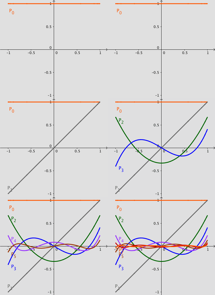
The Legendre polynomials $P_n(x)$ are solutions to the Legendre differential equation:

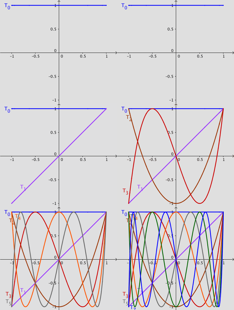
The Chebyshev polynomials $T_n(x)$ are solutions to the Chebyshev differential equation:

Since the Legendre and Chebyshev polynomials are orthogonal functions on the interval $[-1,1]$ with respect to the weights functions
The following simulation shows partial sums of least squares approximations of continuous functions using:
Things to try:
Remark: Notice that the approximation is INCORRECT since the first three coefficients are zero by default in the simulation. Calculate the CORRECT coefficients, rounded to two decimals places, and enter these values in the simulation.
For example, the Legendre approximation of the default function $0.7|x|$ are: $a_0=0.35$, $a_1=0$, $a_2=0.66$. Type these values in the simulation.
The following file contains activities and problems associated with the simulations.